The Amount of Time a Neuron Must Wait Before It Is Able to Fire Again Is Known as

Theexponential distribution is frequently concerned with the amount of time until some specific consequence occurs. For case, the amount of fourth dimension (beginning now) until an convulsion occurs has an exponential distribution. Other examples include the length, in minutes, of long distance business concern telephone calls, and the amount of time, in months, a car battery lasts. It can be shown, too, that the value of the modify that you have in your pocket or purse approximately follows an exponential distribution.

Values for an exponential random variable occur in the post-obit way. There are fewer big values and more small values. For instance, the amount of coin customers spend in one trip to the supermarket follows an exponential distribution. There are more people who spend pocket-sized amounts of coin and fewer people who spend large amounts of money.

The exponential distribution is widely used in the field of reliability. Reliability deals with the amount of fourth dimension a production lasts.

Example

PermitX = amount of time (in minutes) a postal clerk spends with his or her customer. The time is known to have an exponential distribution with the average amount of time equal to four minutes.

X is a continuous random variable since fourth dimension is measured. It is given that μ = 4 minutes. To do whatever calculations, you must know m, the disuse parameter.

[latex]{m}=\frac{i}{\mu}[/latex]. Therefore, [latex]{chiliad}=\frac{i}{four}={0.25}[/latex]

The standard deviation, σ, is the same every bit the mean. μ = σ

The distribution notation is X ~ Exp(m). Therefore, X ~ Exp(0.25).

The probability density function is f(x) = me ^–mx . The number e = 2.71828182846… It is a number that is used often in mathematics. Scientific calculators take the key "e^x ." If y'all enter one for x, the computer will display the value east.

The bend is:

f(10) = 0.25due east ^–0.25ten where x is at least zero and 1000 = 0.25.

For example, f(5) = 0.25east ^−(0.25)(v) = 0.072. The postal clerk spends five minutes with the customers. The graph is equally follows:

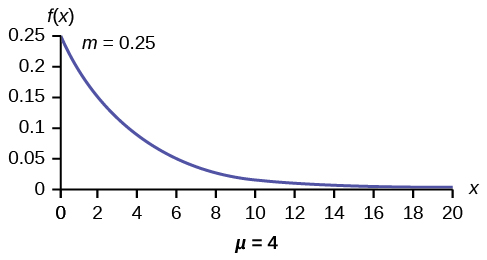
Find the graph is a declining curve. When x = 0,

f(x) = 0.25e ^(−0.25)(0) = (0.25)(1) = 0.25 = one thousand. The maximum value on the y-axis is grand.

Try It

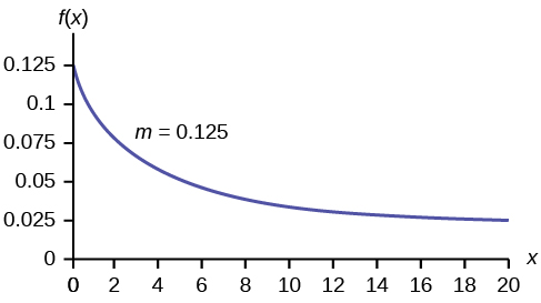
The amount of time spouses shop for anniversary cards can be modeled by an exponential distribution with the average amount of time equal to viii minutes. Write the distribution, country the probability density function, and graph the distribution.

Solution:

Ten ~ Exp(0.125); f(x) = 0.125e^–0.125x ;

 Instance

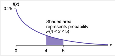
Using the information in example 1, find the probability that a clerk spends four to five minutes with a randomly selected customer.

The curve is:

X ~ Exp(0.125); f(x) = 0.125e^–0.125x

a) Find P(4 < 10 < five).

Solution:

The cumulative distribution function (CDF) gives the area to the left.

P(x < x) = one – e^–mx

P(x < 5) = 1 – e(–0.25)(5) = 0.7135 and P(10 < 4) = i – e ^(–0.25)(4) = 0.6321

You lot tin can exercise these calculations hands on a calculator.

 The probability that a postal clerk spends four to v minutes with a randomly selected customer is P(four < ten < 5) = P(10 < 5) – P(10 < four) = 0.7135 − 0.6321 = 0.0814.

On the home screen, enter (ane – e^(–0.25*five))–(1–e^(–0.25*4)) or enter e^(–0.25*4) – e^(–0.25*5).

b) Half of all customers are finished within how long? (Find the fifty^th percentile)

Solution:

Find the 50^th percentile.

P(x < yard) = 0.50, k = 2.8 minutes (computer or computer)

One-half of all customers are finished within two.eight minutes.

You can also do the calculation as follows:

P(x < k) = 0.50 and P(x < k) = ane –due east ^{–0.25one thousand}

Therefore, 0.l = 1 − e ^−0.25k and e ^−0.25k = i − 0.50 = 0.5

Take natural logs: ln(e ^–0.25k ) = ln(0.l). So, –0.25k = ln(0.50)

Solve for thou:  [latex]{grand}=\frac{ln0.50}{-0.25}={0.25}=ii.8[/latex] minutes

c) Which is larger, the hateful or the median?

Solution:

From role b, the median or l^thursday percentile is ii.eight minutes. The theoretical mean is iv minutes. The mean is larger.

 Example

The number of days ahead travelers purchase their airline tickets can exist modeled by an exponential distribution with the average amount of time equal to 15 days. Find the probability that a traveler volition purchase a ticket fewer than x days in advance. How many days do half of all travelers expect?

Solution:

P(10 < 10) = 0.4866

50^th percentile = 10.40

Instance

On the boilerplate, a certain calculator part lasts x years. The length of time the computer part lasts is exponentially distributed.

 a) What is the probability that a reckoner part lasts more than seven years?

Solution:Permit x = the amount of fourth dimension (in years) a computer part lasts.

[latex]\mu = {10}[/latex] so yard = [latex]\frac{1}{\mu} = \frac{1}{10}={0.10}[/latex]
P(x > 7). Draw the graph.

P(x > 7) = ane – P(ten < vii).

Since P(X < x) = 1 –e^–mx and so P(Ten > x) = 1 –(ane –e^–mx ) = e^-mx

P(x > seven) = due east ^(–0.1)(7) = 0.4966. The probability that a computer office lasts more than than seven years is 0.4966.

On the home screen, enter due east^(-.1*seven).

b) On the average, how long would five reckoner parts concluding if they are used one later another?

Solution:

On the average, one computer role lasts 10 years. Therefore, five computer parts, if they are used i right after the other would final, on the boilerplate, (5)(x) = fifty years.

c) Eighty per centum of computer parts terminal at well-nigh how long?

Solution:

Find the 80^thursday percentile. Depict the graph. Let k = the 80^th percentile.

Solve for k: [latex]{k}=\frac{ln(1-0.80)}{-0.1}={16.1}[/latex]

Eighty percent of the reckoner parts final at most sixteen.1 years.

Solution:

Find P(9 < x < 11). Depict the graph.

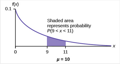
d) What is the probability that a estimator part lasts betwixt nine and xi years?

Solution:

P(9 < ten < 11) = P(x < eleven) – P(10 < 9) = (1 – e ^{(–0.ane)(11)}) – (1 – e ^(–0.1)(9)) = 0.6671 – 0.5934 = 0.0737. The probability that a computer part lasts between nine and 11 years is 0.0737.

Example

Suppose that the length of a telephone telephone call, in minutes, is an exponential random variable with decay parameter = 1 12 . If another person arrives at a public telephone just before yous, find the probability that you will take to wait more than five minutes. Let X = the length of a phone call, in minutes.

What is m, μ, and σ? The probability that yous must expect more than than v minutes is _______ .

Solution:

thou =  [latex]\frac{1}{12}[/latex]

[latex]\mu [/latex] = 12

[latex]\sigma [/latex] = 12

P(ten > v) = 0.6592

Example

The time spent waiting between events is oftentimes modeled using the exponential distribution. For case, suppose that an average of xxx customers per hour arrive at a store and the time between arrivals is exponentially distributed.

1. On average, how many minutes elapse between ii successive arrivals?
2. When the store first opens, how long on average does information technology take for iii customers to arrive?
3. Later on a client arrives, notice the probability that it takes less than ane infinitesimal for the next customer to arrive.
4. After a customer arrives, find the probability that it takes more than five minutes for the next customer to go far.
5. Seventy pct of the customers arrive within how many minutes of the previous client?
6. Is an exponential distribution reasonable for this situation?

Solutions:

1. Since we await 30 customers to arrive per 60 minutes (hr), we expect on average one customer to arrive every two minutes on average.
2. Since one customer arrives every two minutes on average, it will have six minutes on average for three customers to get in.
3. Let X = the time betwixt arrivals, in minutes. By part a, μ = ii, so m = 1 2 = 0.five.
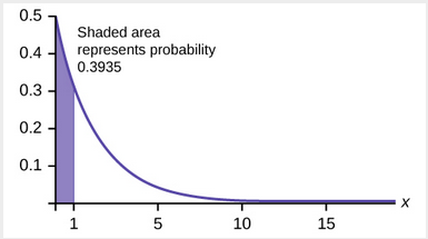
   Therefore, X ∼ Exp(0.five).The cumulative distribution office is P(X < x) = 1 – eastward(–0.5x) ^e .Therefore P(X < 1) = one – east^(–0.v)(1) ≈ 0.3935

4. 

5. P(X > 5) = 1 – P(Ten < five) = 1 – (1 – due east ^(–v)(0.5)) = e^–ii.5 ≈ 0.0821.

6. 
7. We desire to solve 0.seventy = P(X < ten) for x.
   Substituting in the cumulative distribution function gives 0.70 = 1 – e ^–0.5x , so that e ^–0.5x = 0.30. Converting this to logarithmic form gives –0.fivex = ln(0.thirty), or x = fifty n ( 0.xxx ) – 0.v ≈ 2.41 minutes.Thus, lxx per centum of customers make it inside ii.41 minutes of the previous customer.
8. This model assumes that a single customer arrives at a time, which may not be reasonable since people might shop in groups, leading to several customers arriving at the same time. Information technology as well assumes that the menstruum of customers does non alter throughout the day, which is non valid if some times of the day are busier than others.

Memorylessness of the Exponential Distribution

In example 1, recall that the amount of fourth dimension between customers is exponentially distributed with a mean of two minutes (X ~ Exp (0.5)). Suppose that five minutes have elapsed since the final customer arrived. Since an unusually long corporeality of time has at present elapsed, information technology would seem to be more likely for a customer to get in within the next infinitesimal. With the exponential distribution, this is not the case–the additional time spent waiting for the next customer does not depend on how much time has already elapsed since the last customer. This is referred to as the memoryless belongings. Specifically, the memoryless property says that

P (Ten > r + t | X > r) = P (Ten > t) for all r ≥ 0 and t ≥ 0

For case, if five minutes has elapsed since the last customer arrived, and then the probability that more than than 1 infinitesimal volition elapse before the next customer arrives is computed by using r = 5 and t = i in the foregoing equation.

P(X > five + 1 | Ten > v) = P(X > 1) = e ( – 0.5 ) ( 1 ) ≈ 0.6065.

This is the aforementioned probability every bit that of waiting more than one minute for a customer to go far afterwards the previous arrival.

The exponential distribution is oftentimes used to model the longevity of an electric or mechanical device. In example 1, the lifetime of a sure figurer part has the exponential distribution with a hateful of 10 years (10 ~ Exp(0.one)). The memoryless belongings says that knowledge of what has occurred in the past has no issue on future probabilities. In this case information technology means that an old role is not whatsoever more likely to break down at any item time than a brand new part. In other words, the part stays as good as new until information technology suddenly breaks. For example, if the part has already lasted ten years, so the probability that it lasts another seven years is P(X > 17|X > ten) =P(X > 7) = 0.4966.

Example

Refer to example 1, where the time a postal clerk spends with his or her client has an exponential distribution with a mean of four minutes. Suppose a customer has spent four minutes with a postal clerk. What is the probability that he or she will spend at to the lowest degree an additional iii minutes with the postal clerk?

The disuse parameter of Ten is g = 14 = 0.25, then 10 ∼ Exp(0.25).
The cumulative distribution function is P(X < x) = i – e–0.25x. We want to find P(Ten > vii|X > 4). The memoryless holding says that P(Ten > 7|X > 4) = P (10 > 3), and so we but need to find the probability that a customer spends more than than three minutes with a postal clerk.
This is P(X > 3) = ane – P (X < 3) = 1 – (1 – east–0.25⋅iii) = e–0.75 ≈ 0.4724.

Relationship between the Poisson and the Exponential Distribution

There is an interesting human relationship between the exponential distribution and the Poisson distribution. Suppose that the time that elapses between 2 successive events follows the exponential distribution with a mean of μ units of time. Also assume that these times are independent, pregnant that the time between events is not afflicted by the times betwixt previous events. If these assumptions hold, then the number of events per unit time follows a Poisson distribution with mean λ = 1/μ. Recall that if X has the Poisson distribution with hateful λ, then [latex]P(X=k)=\frac{{\lambda}^{k}{e}^{-\lambda}}{k!}[/latex]. Conversely, if the number of events per unit time follows a Poisson distribution, then the corporeality of time between events follows the exponential distribution. (k! = 1000*(g-1*)(k–ii)*(thou-three)…3*2*1)

Example

At a police station in a large city, calls come in at an average rate of four calls per infinitesimal. Assume that the time that elapses from one call to the next has the exponential distribution. Have notation that we are concerned only with the charge per unit at which calls come in, and we are ignoring the time spent on the phone. We must also assume that the times spent between calls are independent. This ways that a particularly long delay between 2 calls does not mean that there will exist a shorter waiting period for the next phone call. We may and so deduce that the full number of calls received during a time catamenia has the Poisson distribution.

1. Notice the average fourth dimension between two successive calls.
2. Discover the probability that afterwards a call is received, the next call occurs in less than 10 seconds.
3. Find the probability that exactly 5 calls occur within a infinitesimal.
4. Detect the probability that less than 5 calls occur within a infinitesimal.
5. Find the probability that more than 40 calls occur in an eight-minute period.

Solutions:

1. On boilerplate there are four calls occur per minute, then xv seconds, or [latex]\frac{xv}{sixty} [/latex]= 0.25 minutes occur between successive calls on boilerplate.
2. Let T = time elapsed betwixt calls. From office a, [latex]\mu = {0.25} [/latex], and then yard = [latex]\frac{1}{0.25} [/latex] = iv. Thus, T ~ Exp(4).  The cumulative distribution office is P(T < t) = 1 – e ^–4t . The probability that the next call occurs in less than x seconds (ten seconds = 1/half dozen infinitesimal) is P(T < [latex]\frac{i}{6}[/latex]) = 1 –  [latex]{e}^{-4\frac{1}{6}} \approx{0.4866} [/latex]
3. Allow X = the number of calls per minute. As previously stated, the number of calls per infinitesimal has a Poisson distribution, with a hateful of four calls per infinitesimal. Therefore, Ten ∼ Poisson(4), and then P(10 = 5) = [latex]\frac{{iv}^{5}{e}^{-4}}{5!}\approx[/latex] 0.1563. (v! = (5)(4)(3)(ii)(1))
4. Proceed in mind that X must be a whole number, so P(X < 5) = P(X ≤ iv).

   To compute this, we could accept P(10 = 0) + P(X = 1) + P(X = 2) + P(X = 3) + P(X = 4).

   Using engineering science, we meet that P(Ten ≤ 4) = 0.6288.

5. Let Y = the number of calls that occur during an eight minute period.

   Since there is an boilerplate of four calls per minute, in that location is an average of (8)(iv) = 32 calls during each viii minute period.

   Hence, Y ∼ Poisson(32). Therefore, P(Y > 40) = 1 – P (Y ≤ 40) = 1 – 0.9294 = 0.0707.

Concept Review

If X has an exponential distribution with mean [latex]\mu[/latex] then the decay parameter is [latex]g =\frac{one}{\mu}[/latex], and nosotros write X ∼ Exp(m) where 10 ≥ 0 and g > 0 . The probability density part of 10 is f(x) =me^-mx (or equivalently [latex]f(x)=\frac{one}{\mu}{e}^{\frac{-x}{\mu}}[/latex].The cumulative distribution function of X is P(X≤ x) = 1 – e ^–mx .

The exponential distribution has the memoryless property, which says that future probabilities do not depend on any past information. Mathematically, it says that P(Ten > x + k|X > x) = P(X > k).

If T represents the waiting time betwixt events, and if T ∼ Exp(λ), then the number of events 10 per unit of measurement time follows the Poisson distribution with mean λ. The probability density function of [latex]P\left(10=k\correct)=\frac{\lambda^{k}}{e^{-\lambda}}g![/latex]. This may be computed using a TI-83, 83+, 84, 84+ reckoner with the control poissonpdf(λ, k). The cumulative distribution role P(10 ≤ yard) may be computed using the TI-83, 83+,84, 84+ figurer with the command poissoncdf(λ, grand).

Formula Review

Exponential: 10 ~ Exp(m) where one thousand = the decay parameter

• pdf: f(x) = grand[latex]{e}^{-mx}[/latex] where ten ≥ 0 and grand > 0
• cdf: P(Ten ≤ x) = 1 –[latex]{e}^{-mx}[/latex]
• mean [latex]\mu = \frac{1}{m}[/latex]
• standard deviation σ = µ
• percentile, 1000: k = [latex]\frac{ln(\text{AreaToTheLeftOfK})}{-m}[/latex]
• Additionally
  • P(X > x) = e ^(–mx)
  • P(a < X < b) = e ^(–ma) – e ^(–mb)
• Memoryless Property: P(10 > 10 + g|10 > 10) = P (X > g)
• Poisson probability:P ( X = k ) =[latex]\frac{{\lambda}^{k}{e}^{-\lambda}}{m!}[/latex] with hateful [latex]\lambda[/latex]
• thou! = 1000*(k-1)*(k-2)*(thousand-iii)…3*2*1

References

Data from the United States Demography Agency.

Data from World Earthquakes, 2013. Available online at http://world wide web.world-earthquakes.com/ (accessed June 11, 2013).

"No-hitter." Baseball-Reference.com, 2013. Bachelor online at http://www.baseball game-reference.com/pitcher/No-hitter (accessed June xi, 2013).

Zhou, Rick. "Exponential Distribution lecture slides." Available online at www.public.iastate.edu/~riczw/stat330s11/lecture/lec13.pdf‎ (accessed June 11, 2013).

mintztwoul1969.blogspot.com

Source: https://courses.lumenlearning.com/introstats1/chapter/the-exponential-distribution/

Share this post